In one paragraph. In 1960, Heinz von Foerster, Patricia Mora and Lawrence Amiot published a paper in Science with the title “Doomsday: Friday, 13 November, A.D. 2026”. They fitted the equation N = K / (t0 − t)k to estimates of world population since the time of Christ and found that it fits very well and reaches infinity at t0 = 2026.87 ± 5.50. I re-ran their published equation against the World Bank’s population series for 1960-2025. It tracked reality within about 11% until the mid-1990s. By 2025 it predicts 96 billion people. The real figure is 8.22 billion. The deeper test, which needs no curve fitting at all, is the growth rate: the model needs growth to keep speeding up as population rises, and real growth peaked at 2.12% a year in 1963 and has fallen ever since. Everything below can be reproduced from one ZIP file.
A date with a deadline
Eight days from now is Friday 13 November 2026. If you have seen it described online as “the day the world ends”, this is where it comes from.
The claim is not from a prophet or a calendar. It comes from a respected journal, from a respected scientist, and from a very simple piece of mathematics. That makes it a good story, and an even better exercise: a published prediction with a date on it, written 66 years ago, that we can now check against what actually happened.
So I treated it as a small reproduction study. I rebuilt the model, collected the data, ran the original equation forward, and asked three questions:
- Did the model fit the evidence the authors had in 1960?
- How well did it predict the 65 years that came after?
- If it failed, why, in a way we can measure?
1. The paper
The paper is von Foerster, Mora and Amiot (1960), Science 132(3436): 1291-1295 (doi:10.1126/science.132.3436.1291). Heinz von Foerster was a physicist and one of the founders of cybernetics, and ran the Biological Computer Laboratory at the University of Illinois. The subtitle says the whole thing: “At this date human population will approach infinity if it grows as it has grown in the last two millennia.”
The authors collected 24 estimates of world population from the literature, ranging from the time of Christ to 1958, removed estimates that looked like copies of each other, left out 1958 itself, and fitted a curve by least squares. Their published result, which is all we need to test them, is:
N(t) = 1.79 × 10¹¹ / (2026.87 − t)0.99
with K = (1.79 ± 0.14) × 1011, k = 0.990 ± 0.009 and t0 = 2026.87 ± 5.50 years, and a root-mean-square error of about 7% over their points.
As (2026.87 − t) shrinks towards zero, N grows without limit. That is the “doomsday”: not a prediction that everybody dies, but that the formula describing two thousand years of human history stops making sense at that moment.
2. The mathematics, step by step
Most growth stories start with the exponential. If each person, on average, adds a fixed fraction a of a person per year, then
dN/dt = a · N → N(t) = N0 ea t
Exponential growth is fast, but it never reaches infinity in finite time. Its doubling time is fixed: ln 2 / a.
Von Foerster’s idea was that a is not fixed. More people means more cooperation, more ideas and more ways to beat famine and disease, so the growth rate itself rises with population. They wrote it as a = a0 · N1/k. Put that into the growth equation and you get
dN/dt = a0 · N1 + 1/k
Separate the variables and integrate:
∫ N−1 − 1/k dN = ∫ a0 dt → k · N−1/k = a0 (t0 − t) → N(t) = K / (t0 − t)k, with K = (k / a0)k
The constant of integration, t0, is the date at which N becomes infinite. Mathematicians call this a finite-time singularity. Any growth law where the rate rises faster than linearly with N has one.
Two more consequences fall out of the same equation, and both are testable:
- Growth rate. r = d(ln N)/dt = k / (t0 − t). The percentage growth rate must keep rising, and it is tied to population: r = k · (N / K)1/k.
- Doubling time. Solving N(t + Δ) = 2N(t) gives Δ = (1 − 2−1/k) · (t0 − t), which is about half of the time remaining for k = 0.99. Each doubling takes half as long as the one before.
Why 2026.87 became “Friday 13 November”
0.87 of a year is day 318 of 2026, which is Saturday 14 November. Friday 13 November is day 317 (2026.866). Rounded to two decimals, the paper’s own number fits both days, and with an uncertainty of ±5.5 years (anywhere from 2021 to 2032) the choice of Friday the 13th was a joke the data allowed, not a result.
3. The data
I used two public datasets. Both are in the download, and both can be fetched again from their sources.
| Period | Dataset | Source | Licence |
|---|---|---|---|
| AD 1 to 1955 | 104 historical estimates from 8 authors (Deevey, McEvedy & Jones, Durand, Clark, Biraben, Blaxter, UN, Kremer) | Appendix of J. E. Cohen, How Many People Can the Earth Support? (Norton, 1995), packaged by datahub.io (raw CSV) | ODC PDDL (public domain) |
| 1960 to 2025 | World population, total (SP.POP.TOTL), country code WLD | World Bank, World Development Indicators (API); copy taken 5 November 2026, series last updated 8 October 2026; based on the UN World Population Prospects | CC BY 4.0 |
One honest caveat before any results. The 1960 paper shows its 24 estimates only as dots on a chart, with reference numbers, not as a table of values. I could not recover the exact 24 numbers, so I did two things instead. I test the paper’s published equation and parameters directly, which needs no data of theirs at all. And for the pre-1960 evidence I use Cohen’s compilation, which covers the same span from the same kinds of sources (some published after 1960). Where that choice changes an answer, I say so.
4. What the re-run shows
Step 1. In 1960, the law looked excellent
 ↓ Download PNG
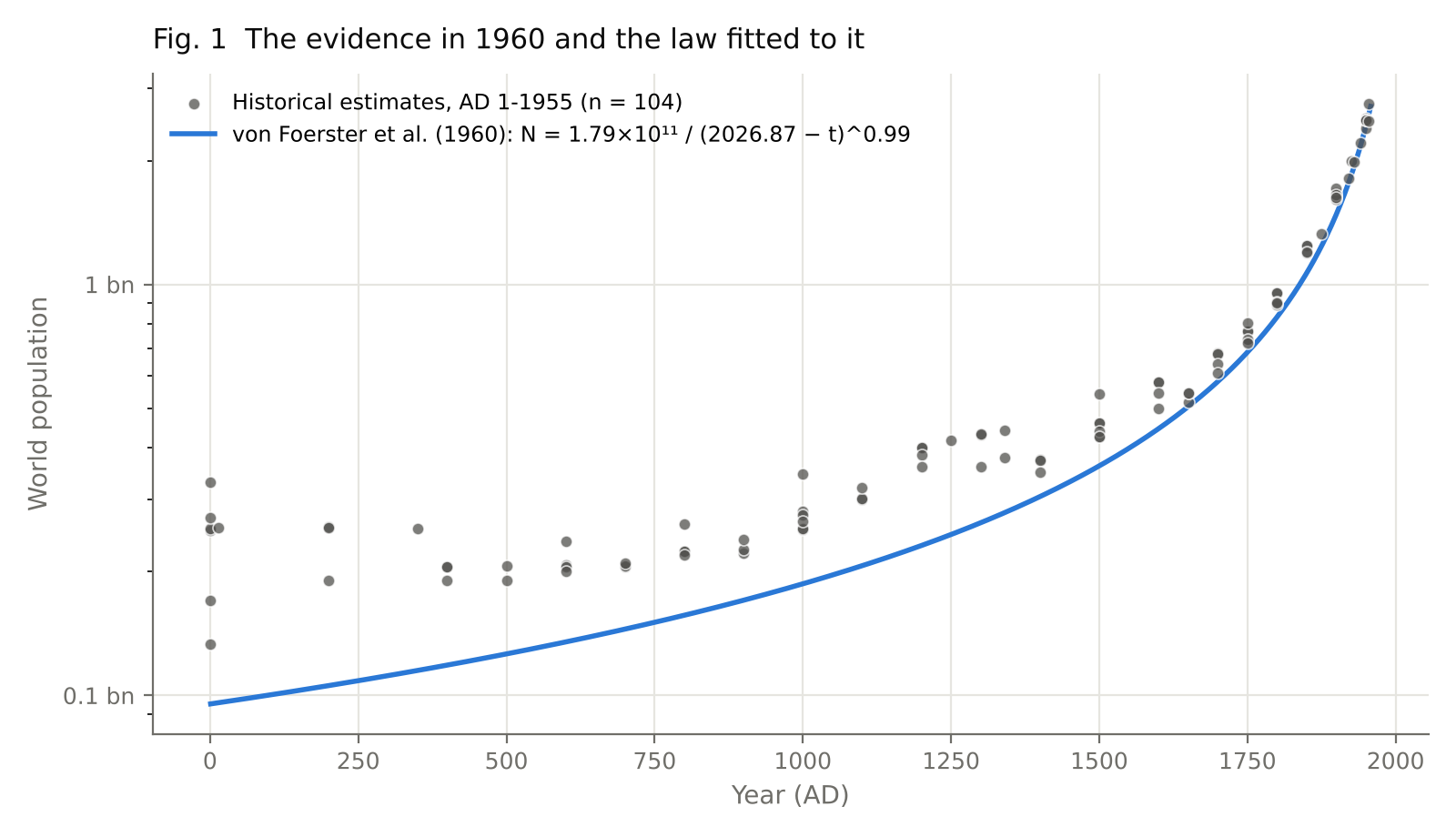
From 1500 to 1955, the 1960 law sits within about 13% (RMS of the log error, 0.134) of the 52 estimates in that period. That is not far from the paper’s own 7%, given that these estimates often differ from each other by more than that. Before 1500 the law undershoots: it puts the world at about 95 million in AD 1, where modern estimates say 170-330 million. Ancient population is very uncertain, but it is a first sign that one equation for all of history was an act of faith.
 ↓ Download PNG
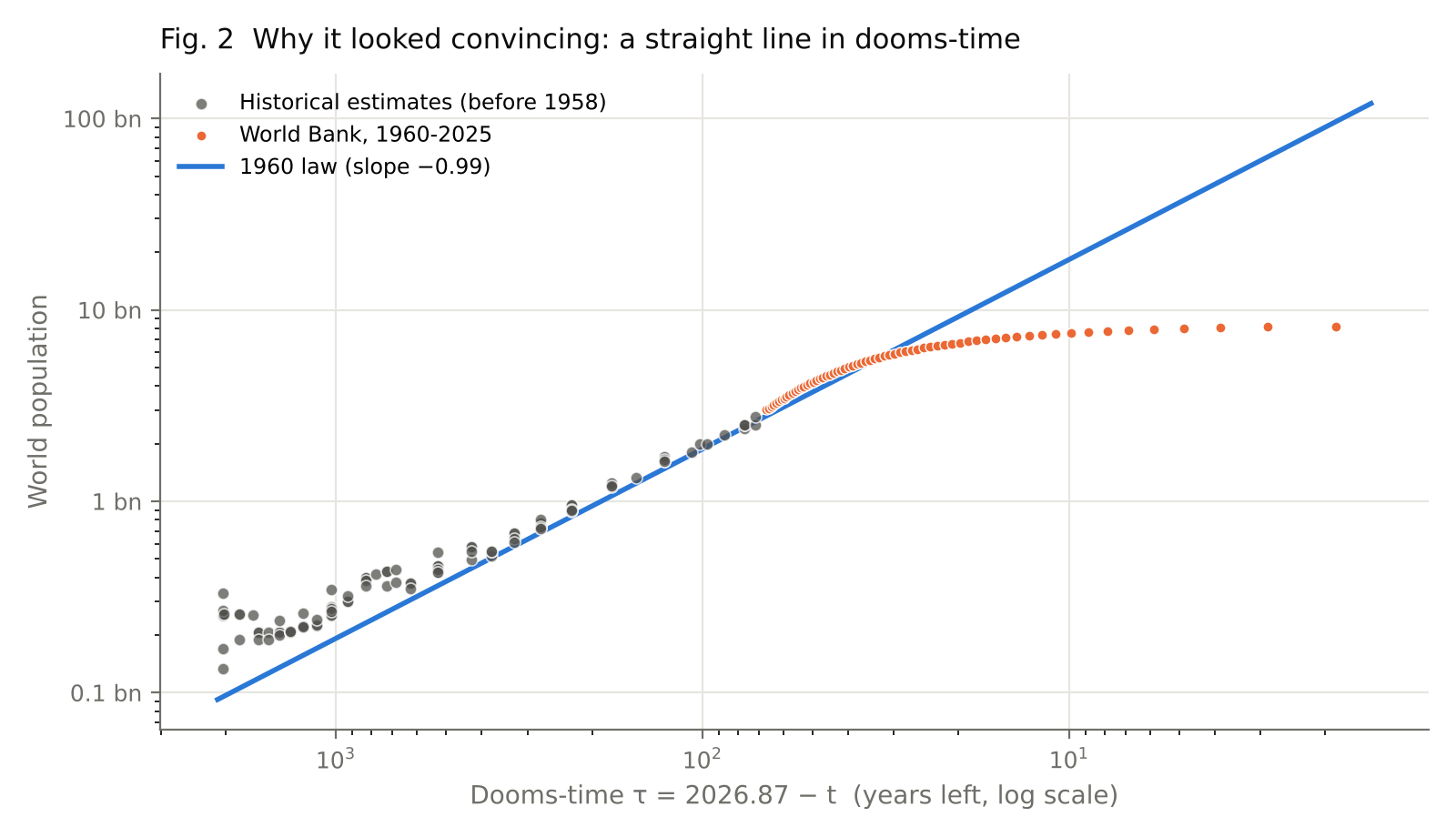
Figure 2 is the authors’ own way of looking at it, and it shows why the idea was so persuasive. Plot population against the years left until doomsday, both on log scales, and two thousand years of history fall on a straight line. The orange dots are what happened next: they follow the line for about 30 years, then turn flat.
Step 2. Refitting the same law: the date depends on the data
I refitted N = K / (t0 − t)k by least squares on ln N, so each point counts by its relative error:
| Data used | k | t0 (doomsday) | RMS log error |
|---|---|---|---|
| The paper (24 estimates, AD 0-1957) | 0.990 | 2026.87 ± 5.50 | about 0.07 |
| All 104 Cohen estimates, AD 1-1955 | 0.676 | 1989.6 ± 6.1 (bootstrap 95%: 1980.7 to 1999.6) | 0.140 |
| Cohen estimates, 1500-1955 only | 0.881 | 2021.6 ± 8.5 | 0.057 |
The hyperbola fits every version of the data, but the date it gives moves by 30 years depending on which estimates of ancient population go in. That is the first scientific problem: t0 is an extrapolation far outside the data, and a fit with three free parameters can be very sure about the shape of the past and very unsure about where the singularity sits.
Step 3. The prediction against 65 years of reality
 ↓ Download PNG
| Year | Observed (World Bank) | 1960 law | Law ÷ observed |
|---|---|---|---|
| 1960 | 3.02 bn | 2.79 bn | 0.92 |
| 1970 | 3.68 bn | 3.28 bn | 0.89 |
| 1980 | 4.44 bn | 3.97 bn | 0.89 |
| 1990 | 5.30 bn | 5.03 bn | 0.95 |
| 2000 | 6.16 bn | 6.88 bn | 1.12 |
| 2010 | 7.00 bn | 10.91 bn | 1.56 |
| 2020 | 7.85 bn | 26.56 bn | 3.38 |
| 2025 | 8.22 bn | 96.32 bn | 11.72 |
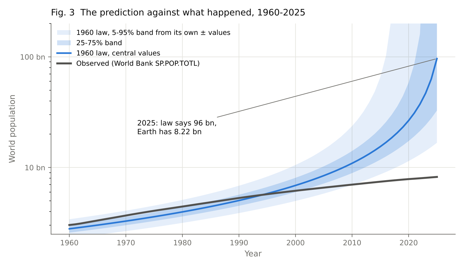
Credit where it is due: for 35 years the law was within about 11% of reality, a little low, which is a remarkable run for a two-line formula. It caught up with the real population in 1995, overshot by more than its own 7% error from 1999, was double reality by 2015, and more than ten times reality in 2025.
Monte Carlo test. Perhaps the central values were just unlucky? I drew 20,000 sets of (K, k, t0) from the paper’s own ± uncertainties (normal distributions, fixed random seed). In 37.5% of the draws doomsday has already happened before 2025. In the rest, the median 2025 population is 40 billion, and the 5-95% range is 15 to 386 billion. Only 0.04% of all draws come within 7% of the real 8.22 billion. The paper’s error bars do not rescue it.
Step 4. The decisive test: the growth rate
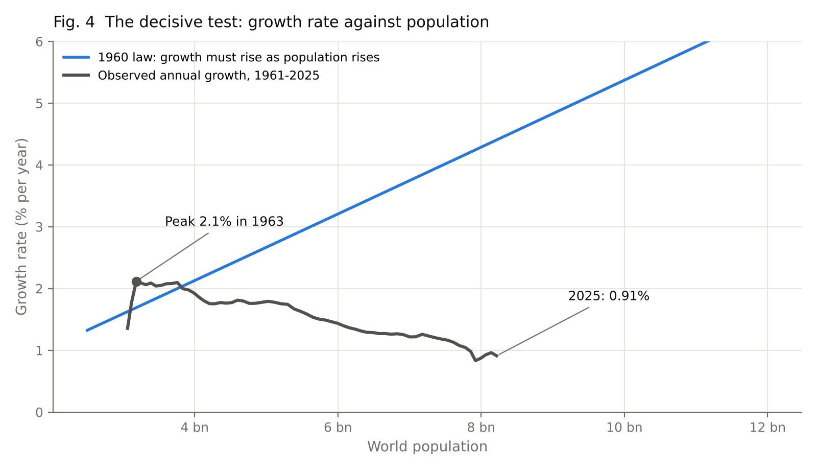
Curve fits can always be argued about. The growth rate cannot. The model says, without any fitting, that the growth rate must rise with population: r = k · (N / K)1/k.
 ↓ Download PNG
Real growth rose until 1963, when it reached 2.12% a year, and has fallen almost every decade since, to 0.91% a year in 2025. The 1960 law, at 2025’s date, requires 52.9% a year. The two curves go in opposite directions. This is the cleanest evidence that the assumption behind the model, “the more of us there are, the faster we grow”, stopped being true in the early 1960s.
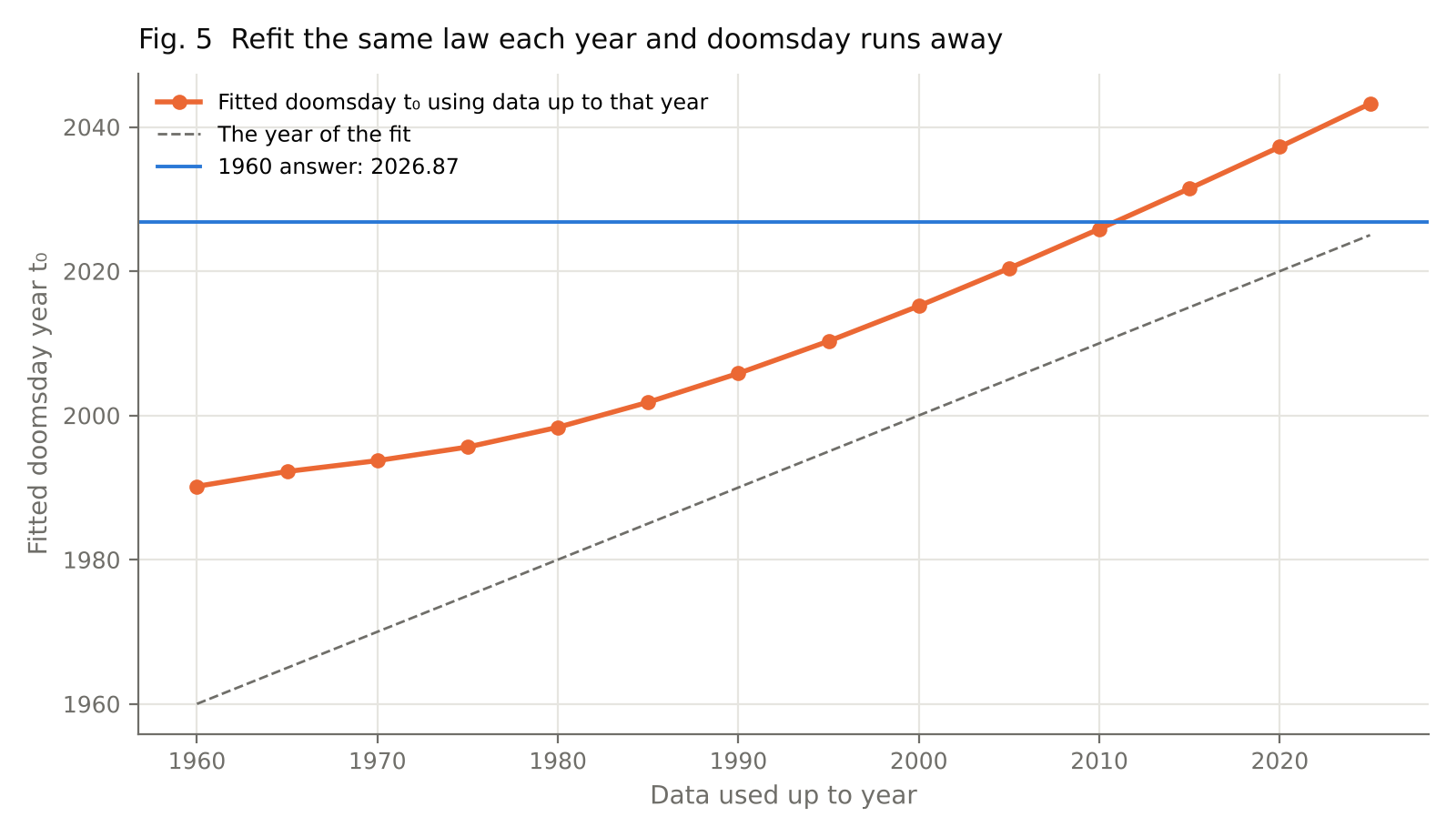
Step 5. Refit every five years, and doomsday runs away
 ↓ Download PNG
Suppose a believer kept the model and simply refitted it as new data came in. With the historical estimates plus World Bank data up to 1960, doomsday is 1990. With data to 1990, it is 2006. With data to 2010, it is 2026. With data to 2025, it is 2043, and the fit is getting worse (RMS log error up from 0.139 to 0.176). The singularity recedes almost as fast as we approach it. A model whose central prediction moves with every new data point is not predicting anything.
Step 6. What does fit after 1960
 ↓ Download PNG
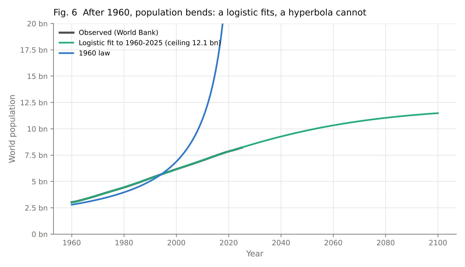
The post-1960 data bend. A simple logistic (S-shaped) curve fitted to 1960-2025 matches the World Bank series to within 0.24% RMS, with a ceiling of about 12.1 billion. I show this only to make the shape visible, not as a forecast. Real projections use births, deaths and migration by age. The UN’s World Population Prospects 2024 projects a peak of about 10.3 billion in the mid-2080s, followed by a slow decline.
5. So why was it wrong?
The mathematics was right. The assumption was not.
The hyperbolic law is a good description of a world in which more people mean more technology, and more technology means faster growth. Economists later took that idea seriously: Michael Kremer (1993) showed that a model of population and technology feeding each other explains the long era of ever-faster growth, from one million BC until the demographic transition set in. The physicist Sergey Kapitza (1996) built a theory around the same hyperbola and argued that it must give way to a stable population, with the change happening around the end of the 20th century.
What broke it is the demographic transition. As child mortality fell, education spread (especially for women), contraception became available and people moved to cities, families became smaller. Birth rates fell after death rates, so growth rose for a while and then fell. Population is still rising today because of momentum (a large generation of young adults), but the rate is less than half its 1963 peak.
The model had no term for any of that. It extrapolated a feedback loop that was real for two thousand years and assumed it would hold for ever. In data-science language, it was an excellent in-sample fit of a process that changed regime just after the sample ended.
What a student should take from this
- A good fit is not a good forecast. The hyperbola fits 2,000 years beautifully and still fails within 40 years.
- Test the mechanism, not just the curve. The growth-rate test (Fig. 4) needs no fitting and settles the question.
- Watch the parameter you care about. t0 moved by 30 years with a change of input data and by 53 years as new data arrived. Extrapolated parameters deserve wide error bars.
- Respect the authors. Von Foerster and colleagues were explicit, in the subtitle itself, that this was what would happen if growth continued as it had. The conditional was the point.
6. Reproduce it yourself
Everything in this article comes from one Python script. You can run it in about 15 seconds on any laptop.
Step 1. Get the files
Either download everything in one go, doomsday-1960.zip (code, data, figures and my results), or get each file:
- doomsday.py, the analysis script
- requirements.txt, the four Python packages it needs
- README.md, the sources and licences
- cohen1996_historical_estimates.csv and worldbank_SP.POP.TOTL_WLD.csv, the data, in a folder called
data
Step 2. Install Python and the packages
Install Python 3.10 or newer from python.org. Then, in a terminal inside the unzipped folder:
python -m venv .venv
source .venv/bin/activate        # on Windows: .venv\Scripts\activate
pip install -r requirements.txt
Step 3. Run it
python doomsday.pyTo prove to yourself that I didn’t edit the data, fetch both datasets fresh from their sources first:
python doomsday.py --downloadStep 4. Check your numbers against mine
The script prints every number in this article. Compare it with my output in results/run-output.txt. The first lines should read:
Historical estimates: 104 points from 9 sources, years 1-1955
World Bank series: 66 years, 1960-2025

[1] t0 = 2026.87 -> Saturday 14 November 2026 (±1 s.e.: 2021.37 to 2032.37)
(Nine “sources” because Cohen splits Durand into a low and a high estimate.) The random seed is fixed at 20261113, so the Monte Carlo and bootstrap results match exactly. If the World Bank revises its series after 5 November 2026, --download can move the last decimal places, which is itself a useful lesson in versioning data.
Your figures appear in figures/ (PNG for slides, SVG and PDF for papers) and the full results in results/results.json.
Step 5. How the script works
Part of doomsday.py | What it does |
|---|---|
load_historical() | Reads Cohen’s table, drops the derived “Average” column, keeps AD 1 to 1957 and turns millions into people |
load_worldbank() | Reads the World Bank series for the whole world (WLD) |
hyperbolic() | The 1960 law, N = K / (t0 − t)k |
fit_hyperbolic() | Least squares on ln N with scipy.optimize.curve_fit, with t0 kept later than the last data point |
Steps 1 to 8 in main() | The date, the in-sample check, the refits and bootstrap, the out-of-sample table, the Monte Carlo, the growth rate, the moving doomsday, and the logistic |
Step 6. Try these yourself
- Change the weighting: fit on N instead of ln N. Which years start to dominate, and what happens to t0?
- Fit only 1650-1955. Does doomsday move closer to 2026?
- Replace the logistic with a model that lets the growth rate fall linearly with time from its 1963 peak. When does it reach zero?
- Download a single country’s series from the World Bank (for example India, IND, or Nigeria, NGA) and repeat Fig. 4. Where is each country in its demographic transition?
Limitations
- The paper’s own 24 data points are not tabulated, so the pre-1960 evidence here is a modern compilation of the same period, not the authors’ exact list.
- The World Bank series is itself a set of model-based estimates (from the UN World Population Prospects), not a headcount. Its year-to-year values can be revised.
- Ancient population estimates are uncertain by a factor of two or more, which is exactly why the fitted t0 is so sensitive to them.
- The logistic curve is shown to make the change of shape visible. It is not a population projection.
References
- von Foerster, H., Mora, P. M. & Amiot, L. W. (1960). Doomsday: Friday, 13 November, A.D. 2026. Science, 132(3436), 1291-1295. doi:10.1126/science.132.3436.1291
- Cohen, J. E. (1995). How Many People Can the Earth Support? New York: W. W. Norton. Data appendix as packaged at datahub.io/core/population-global-historical.
- Cohen, J. E. (1995). Population growth and Earth’s human carrying capacity. Science, 269(5222), 341-346.
- World Bank (2026). Population, total (SP.POP.TOTL), World. World Development Indicators. data.worldbank.org/indicator/SP.POP.TOTL. Accessed 5 November 2026. CC BY 4.0.
- United Nations, Department of Economic and Social Affairs, Population Division (2024). World Population Prospects 2024: Summary of Results. population.un.org/wpp
- Kremer, M. (1993). Population growth and technological change: One million B.C. to 1990. The Quarterly Journal of Economics, 108(3), 681-716. doi:10.2307/2118405
- Kapitza, S. P. (1996). The phenomenological theory of world population growth. Physics-Uspekhi, 39(1), 57-71.
- Johansen, A. & Sornette, D. (2001). Finite-time singularity in the dynamics of the world population, economic and financial indices. Physica A, 294(3-4), 465-502.
How to cite this study
Sulaiman, N. V. (2026). Doomsday, Friday 13 November 2026: re-running a 1960 Science paper against 65 years of real data. nihalsulaiman.com. https://nihalsulaiman.com/blog/doomsday-2026-restudy/
Code: MIT licence. Data: as listed above. If you find a mistake, tell me and I will correct it here with a dated note.